Overview Phase 1 — Data Sourcing Phase 2 — Schema & Load Phase 3 — Diagnostics Phase 4 — Optimization Phase 5 — Backup Phase 6 — Security
Phase 02 — Schema Design & Data Loading

Building the Star Schema

I designed a star schema with 4 dimension tables and 10 fact tables, created the database with utf8mb4 charset and InnoDB storage engine, and loaded 22.7 million rows across all 14 tables using SQL LOAD DATA and Python scripts. Every schema decision is documented with a rationale.

Star Schema 14 Tables 22.7M Rows LOAD DATA INFILE InnoDB utf8mb4

What I Did in Phase 2

The Approach

I chose a star schema because the research question — correlating cancer rates with environmental and lifestyle factors — is fundamentally analytical. Dimension tables hold stable reference data while fact tables hold measurements and events. This separation keeps joins predictable and query patterns clean.

Database Configuration

I created cancer_environment_db with utf8mb4 charset and utf8mb4_unicode_ci collation to support the full Unicode range including special characters in geographic and scientific names. InnoDB was the only storage engine considered — ACID compliance and foreign key support are non-negotiable for a relational database of this complexity.

4
Dimension Tables
10
Fact Tables
22.7M
Total Rows
4.57 GB
Database Size
16
Load Scripts

Design Decisions & Rationale

Star Schema Structure

The schema uses four dimension tables — dim_state, dim_county, dim_year, and dim_water_system — as the stable anchors, with ten fact tables radiating outward for each measurement domain.

Decision 01
Star Schema over Flat Tables
The research question requires joining cancer rates to multiple environmental factors. A star schema makes these joins explicit, eliminates redundancy in dimension data, and makes the analytical query patterns predictable.
Decision 02
dim_county from USDA Census
I built dim_county from the USDA Census of Agriculture rather than a generic county list. Only counties with agricultural activity are included — a documented tradeoff that keeps the dimension grounded in real data rather than forcing artificial joins.
Decision 03
dim_water_system as Dimension
Water systems are modeled as a dimension rather than embedded in fact_water_violations. Each public water system serves a geographic area and has stable attributes — treating it as a dimension enables joining violations to counties and states cleanly.
Decision 04
Surrogate Integer Keys
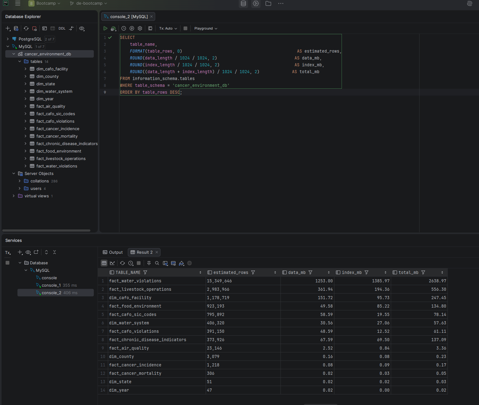
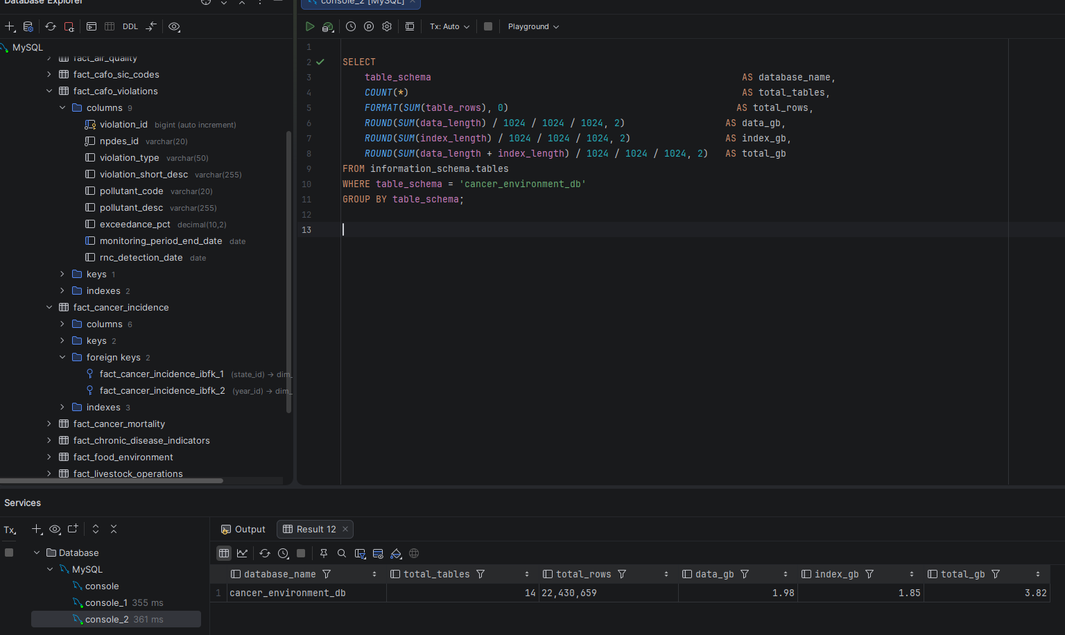
All dimension tables use surrogate AUTO_INCREMENT integer primary keys rather than natural keys. This insulates fact tables from changes in source system identifiers and keeps join columns small and fast for a 22.7M row dataset.
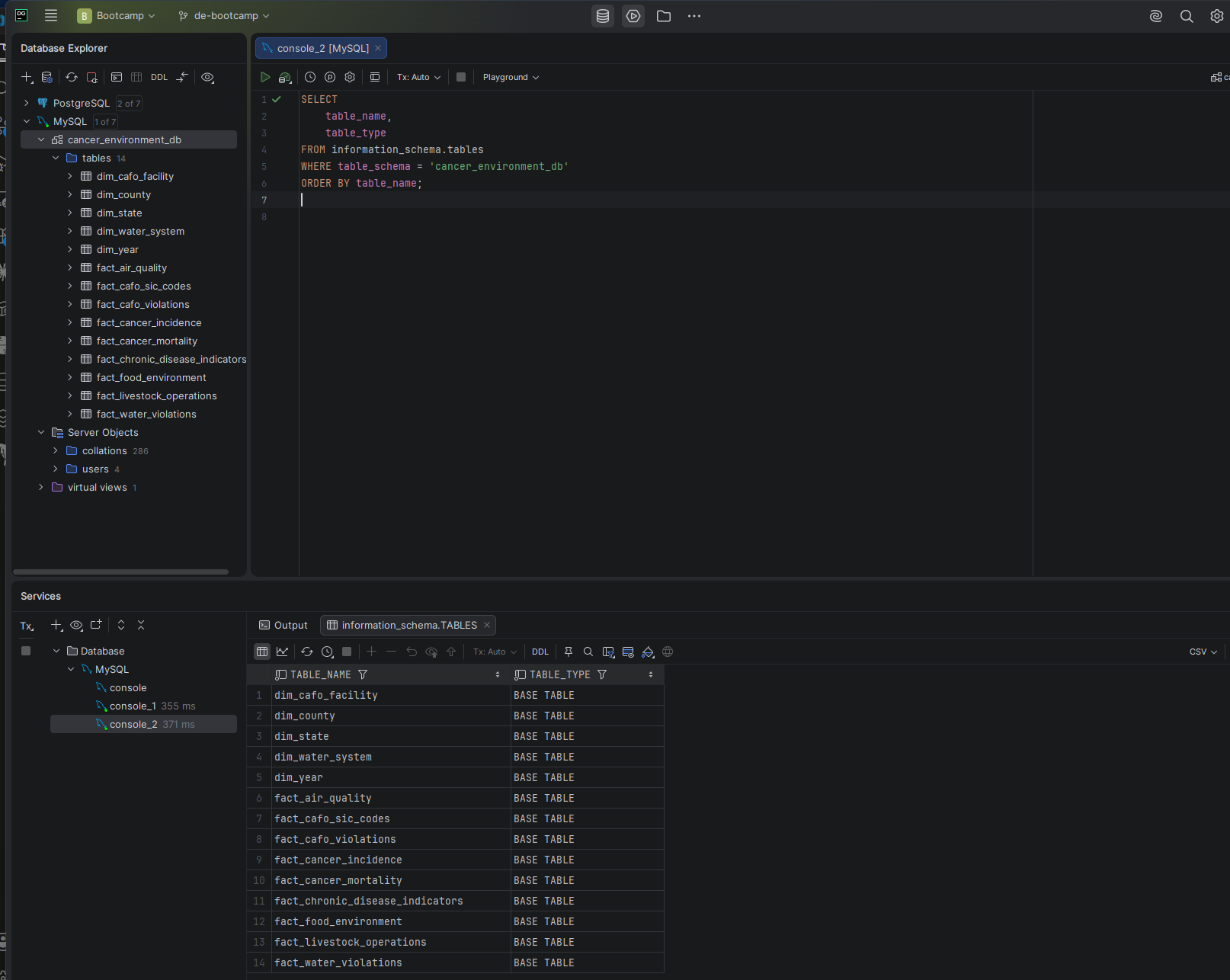
Screenshot — Schema overview in DataGrip
DataGrip database explorer showing all 14 tables in cancer_environment_db
cancer_environment_db — 14 tables visible in the DataGrip database explorer

16 Scripts, 22.7 Million Rows

Load Strategy

I wrote a separate load script for each table — 16 scripts total across Phase 2. Dimension tables were loaded first to establish the reference data, then fact tables in dependency order. For large fact tables like fact_water_violations (15.3M rows) and fact_livestock_operations (3.2M rows), I used LOAD DATA LOCAL INFILE which is significantly faster than row-by-row INSERT.

-- 12_load_water_violations.sql LOAD DATA LOCAL INFILE 'data/raw/water-quality/SDWA_VIOLATIONS_ENFORCEMENT.csv' INTO TABLE fact_water_violations FIELDS TERMINATED BY ',' OPTIONALLY ENCLOSED BY '"' LINES TERMINATED BY '\n' IGNORE 1 ROWS (pwsid, violation_id, violation_category_code, is_health_based_ind, contaminant_code, non_compl_per_begin_date, non_compl_per_end_date);

Load Results by Table

Table Rows Loaded Method
fact_water_violations15,298,031LOAD DATA LOCAL INFILE
fact_livestock_operations3,339,228LOAD DATA LOCAL INFILE
dim_cafo_facility1,188,507LOAD DATA LOCAL INFILE
fact_food_environment930,317LOAD DATA LOCAL INFILE
fact_cafo_sic_codes784,937LOAD DATA LOCAL INFILE
fact_cafo_violations395,599LOAD DATA LOCAL INFILE
dim_water_system433,698Python / LOAD DATA
fact_chronic_disease_indicators375,987LOAD DATA LOCAL INFILE
fact_air_quality23,100Python (23 annual files)
dim_county3,079SQL INSERT
fact_cancer_incidence1,218SQL INSERT
fact_cancer_mortality306SQL INSERT
dim_state51SQL INSERT
dim_year47SQL INSERT
Screenshot — Phase 2 SQL scripts in VS Code
VS Code showing all 16 Phase 2 load scripts
All 16 load scripts organized in sql/phase-2/ — one script per table, dimension tables loaded first

Data Loaded & Verified

Row Count Verification

After all 14 tables were loaded I verified row counts and database size to confirm the load completed correctly and the total size matched expectations for a 22.7 million row dataset.

Screenshot — Table inventory with row counts
Table inventory showing all 14 tables with estimated row counts and sizes
All 14 tables confirmed loaded — row counts and sizes match expected values
Screenshot — Database size summary
Database size summary showing 4.57 GB total across 14 tables
cancer_environment_db — 4.57 GB total, 2.22 GB data + 2.34 GB indexes